 IB Docs (2) Team

D. Analysis
 In this section of the report, you need to describe your results both in words and through tables and graphs. The first step is for you to carry out descriptive statistics.
You should calculate both the central tendency and dispersion if the level of measurement of your data allows it. Depending on your data, you choose the mean, median, or mode. Raw data should not be included here, but must be in an appendix. Only processed data should appear in the results section.
When choosing which measure of central tendency is most appropriate, one of the key considerations is the level of measurement of your data.
Data at the nominal level are the simplest. The data collected are placed in categories and you simply count how many fall into each category; for example, how many participants said 'yes' when asked if they saw 'the broken glass' and how many said ‘no’ (Loftus & Palmer, 1974). Data at the nominal level provide the least amount of information. Only the mode (that is, the most frequent score) can be used as a measure of central tendency. For nominal data, no measure of variability can actually be calculated, but you can discuss the differences in the frequencies of the data.
Ordinal data is often described as “ranked” data. What this means is that the number does not have a true value, but is used to indicate the position in relation to other scores. For example, women who participate in a judo competition are ranked as numbers 1, 2, or 3. We cannot say anything about how much better number 1 did compare with numbers 2 and 3 – only who came in first, second, and third.
Finally, when a number is used but is only a guess, it is also considered ordinal. So, for example, when you estimate the value of 8! in the Tversky & Kahneman study above, the numbers do not have a true value. Therefore, as seen in the sample introduction above, Tversky & Kahneman used the median – the most appropriate measurement for ordinal data. The mode can also be used to describe the data when the data are ordinal. When describing the dispersion of ordinal data, it is best to use the interquartile range [IQR]. The interquartile range is often used to eliminate outliers that may distort the representation of the data.
How to calculate the interquartile range
Suppose you have the following 15 pieces of data from a Likert scale test: 1, 2, 2, 3, 3, 3, 3, 4, 4, 4, 4, 5, 5, 5, 5
The first step is that you have to determine the lower quartile by using the formula (n +1)/4. In this case, it would (15 + 1)/4 – which would give us a value of 4. So, the fourth value on the list of data is the lower quartile. In this case, the value is “3.”
The second step is to determine the upper quartile by using the formula 3(n + 1)/4. In this case, it would be 3(16)/4 – which would give us a value of 12. The twelfth value on the list of data is the upper quartile. In this case, the value is “5.”
The interquartile range is the absolute difference between the upper quartile and the lower quartile. In this case 3 - 5 or “2.”
Data at the interval level are measured on a scale that has precise and equal intervals. Temperature is a good example. If the temperature today is 24 degrees Celsius, you know accurately what the weather is like. However, with interval data, ratios do not make sense. 24 degrees Celsius is not twice as warm as 12 degrees. The mean, median, and mode may be calculated for interval data. To determine the distribution of the data, standard deviation, range, interquartile range, and/or variance may be used.
Ratio. Data at the ratio level have all the characteristics of interval data, plus they have a true zero point—for example, weight in grams is a ratio scale, as something cannot weigh -600 grams. Also, when you ask participants to memorize a list of words – the number that they remember is ratio data. They cannot remember -2 words. Like with interval data, the mean, median, and mode may be calculated. To determine the distribution of the data, standard deviation, range, interquartile range, and/or variance may be used.
The level of measurement will also be important for which inferential statistics you apply.
All these descriptive statistics may be calculated easily using your calculator. You do not need to include the calculation of descriptive statistics in your appendices.
Measures of central tendency and dispersion
| Mean | Very sensitive to outliers (extreme scores). Used with interval and ratio data. |
| Median | Not distorted by outliers. Used with ordinal, interval, and ratio data. |
| Mode | Defined as the most frequently received response. Used with all levels of data. Maybe be distorted by outliers. |
| Range | A measure of dispersion. Easy to calculate, but distorted by outliers. To avoid distortion, use the interquartile range as explained above. |
| Standard deviation | The most sensitive measure of dispersion using all the data. |
The results section should have a chart that clearly states the results of your descriptive statistics - that is, at least one measure of central tendency and one measure of dispersion. In the paragraph that follows this, you should analyze your data. This means that you should describe any trends that were noticed, outliers that may have influenced the data, or other factors that may have influenced the data.
Interpreting your data
In addition to a table with your descriptive statistics and your paragraph that explains those findings, you need to graph the data. When graphing the data, there should be only one graph that reflects your research hypothesis. When making your graph, remember to:
Include a title that reflects your hypothesis.
Label the x and y-axes using operationalized variables. For example - 'time in seconds' on the y-axis and ' congruent' and 'incongruent' on the X-axis. Do not simply label the x-axis as “Groups 1 and 2”.
Since you are comparing two conditions, you should construct a bar graph; do not graph all individual pieces of data. Do not use a histogram as the data is not continuous.
Finally, after your graph, you need to state the findings of your inferential statistical testing and explain the meaning of your results with regard to the null hypothesis.
When choosing a statistical test, there are a few things to consider:
- The level of data: nominal, ordinal, interval, or ratio
- The design: repeated measures or independent samples
- The variance of the two conditions – is there a lot of outliers?
In psychology, the t-test is the most commonly used inferential statistic used to compare the average scores between two small samples. A t-test for dependent groups is used when we have a repeated measures design; a t-test for independent groups is used when we have an independent samples design. We use a t-test when we can assume that the level of measurement of the data is interval or ratio. Often when the data is not clearly interval –for example, when participants estimated the speed in Loftus & Palmer’s (1974) study of leading questions, then a different set of tests is used.
If an independent samples design was used, then the Mann-Whitney U test can be applied to test the significance of the difference between two conditions. If in doubt about whether to use the t-test or the Mann Whitney U, you can use the Mann Whitney U for any test of difference of two independent groups. The Mann Whitney U should always be used with independent samples where you have obtained ordinal data.
If a repeated measures design was used, then the Wilcoxon Signed Ranks test: can be applied to test the significance of the difference between the two conditions. If in doubt about whether to use the t-test or the Wilcoxon Signed Ranks test, you can use the Wilcoxon Signed Ranks test for any test of difference of two dependent groups. The Wilcoxon signed ranks test should always be used with repeated measures designs where you have obtained ordinal data.
The Chi-Squared test is used for nominal data in an independent samples design. For example, when Loftus & Palmer (1974) wanted to see if the number of people who remembered seeing glass was significantly different from those that didn’t, based on their estimation of speed, they applied the chi-squared test.
There are suitable sites on the Internet where you can enter your data once you have chosen the appropriate test. You should print out the calculations and include them in an appendix so that they can be verified by a moderator.
When you have finished calculating your inferential stats, what happens next? You should find what is called the “p-value.” The p-value is the level of probability that your results are due to chance. In psychology, we accept values of p ≤ 0.05, which means that there is a 95% chance that our results are due to the manipulation of the IV and not due to chance. When looking at your results, you should check the p values for a one-tailed test. Based on your p-value, one of two things happens:
If p ≤ 0.05, then you reject the null hypothesis. It appears that chance alone is not the reason for your results; the IV appears to have had an effect on the DV.
If p > 0.05, then you retain the null hypothesis. It appears that you cannot rule out the role of chance, so you cannot state with confidence that the IV has had an effect on the DV.
After you have calculated the p values, you should make a final statement in the analysis section of the report about what this actually means with regard to your hypothesis and your research question. So, for example, if I were testing the Mozart effect with a hypothesis that listening to classical music increases one’s ability to memorize a list of 20 words – and my p-value was 0.09, I would retain the null hypothesis. It appears that classical music does not have an effect on an individual’s ability to memorize a list of 20 words.
Sample analysis
The following analysis is based on the following raw data. Please note that raw data must be located in an appendix and not in the body of the report. It is presented here to help understand the text below.
| Ascending condition | 56, 150, 220, 183, 5800, 820, 20000, 550, 485, 360, 1000, 1200, 4500, 775, 1450, 900 |
| Descending condition | 12500, 10000, 750, 900, 6500, 25000, 13500, 1200, 19000, 16800, 5500, 64000, 3700, 8564, 11500, 10000, 950, 15000 |
In order to analyse the data, I looked at both the median and the mean estimates for each condition.
Table I. Descriptive statistics
| Ascending order | Descending order | |
|---|---|---|
| Mean | 2403.06 | 12520.22 |
| Median | 797.5 | 10000 |
| Interquartile range | 1230 | 10475 |
Because there were outliers in the data for both conditions (see appendix vi), the mean was distorted; so the median was chosen as a measure of central tendency. In addition, because we had some rather extreme outliers, we calculated the interquartile range to determine the dispersion of the data.
The data appears to indicate that the anchor played a role in the estimates given by the participants. There was at least one participant in the ascending condition, however, that estimated 20.000. The interquartile range indicates a larger range of responses in the high anchor condition. The minimum estimate for the ascending condition was 56, whereas it was 750 for the descending condition; the maximum estimate for the ascending condition was 20.000, whereas it was 64000 for the descending condition.
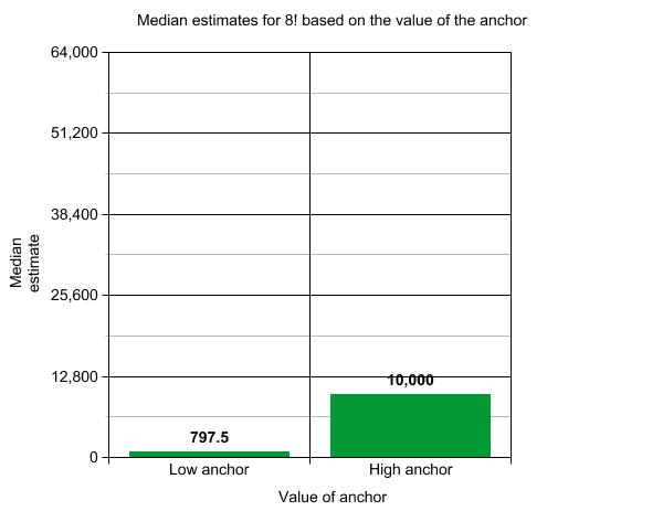
As our data were ordinal, a Mann Whitey U test (see appendix iv) was used to determine whether the difference in the estimates was significant. The Mann-Whitney U test indicated that there was a significant difference between estimates for the higher anchor (Mdn = 10000) and for the lower anchor (Mdn =797.5), U = 41, p = 0.0002. This means that we can reject the null hypothesis. It appears that the value of the anchor plays a significant role in the estimates made by high school mathematics students.
Comments on the sample
The choice of descriptive statistics is explained. There is also a chart showing the descriptive statistics. This is a requirement of the report. There is also one graph that reflects the hypothesis. Both axes are correctly labeled.
The data is discussed - that is, what is interesting about the data or what the data seems to indicate is discussed. The inferential test is identified. The actual calculations of the test must be included in an appendix of the report.
The p-value is stated and interpreted with regard to the hypothesis.
How you are assessed
The following table is the assessment rubric used to award marks for your analysis.
| Marks | Level descriptor |
| 0 |
|
| 1 - 2 |
|
| 3 - 4 |
|
| 5 - 6 |
|
 Twitter
 Facebook
 LinkedIn